STS simulation
This example shows how to
work with Wannier functions in the position representation from Wannier90,
simulate scanning-tunnelling microscopy (STM) and spectroscopy (STS) data.
The Wannier functions used to represent the Hamiltonian (seedname_hr.dat) and those written to file (seedname_0000X.xsf) must be identical (including sign). Hence, the following line in plot.F90 of Wannier90 must be commented out:
wann_func(:, :, :, loop_w) = wann_func(:, :, :, loop_w)/wmod
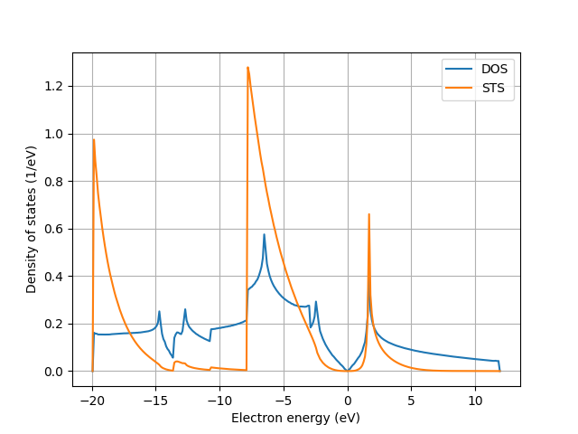
The scanning-tunnelling spectrum is calculated just like the density of states, except that each state is weighted with the square modulus of its overlap with an s orbital located at a chosen position above the sample.
#!/usr/bin/env python3
# Copyright (C) 2017-2026 elphmod Developers
# This program is free software under the terms of the GNU GPLv3 or later.
import elphmod
import matplotlib.pyplot as plt
import numpy as np
comm = elphmod.MPI.comm
info = elphmod.MPI.info
nk = 72
tip = np.array([0.0, 0.0, 12.0]) # tip position (bohr)
V = 1.0 # sample bias (eV)
info('Set up and diagonalize Wannier Hamiltonian')
el = elphmod.el.Model('graphene', read_xsf=True, normalize_wf=True,
check_ortho=True)
e, U, order = elphmod.dispersion.dispersion_full_nosym(el.H, nk,
vectors=True, order=True)
e -= elphmod.el.read_Fermi_level('scf.out')
info('Set up Bravais lattice vectors')
pwi = elphmod.bravais.read_pwi('scf.in')
a = elphmod.bravais.primitives(**pwi, bohr=True)
info('Calculate density of states')
w, dw = np.linspace(e.min(), e.max(), 300, retstep=True)
DOS = sum(elphmod.dos.hexDOS(e[:, :, n])(w) for n in range(el.size))
info('Determine indices of unit-cell corners and vertical tip position')
def indices(point):
return np.unravel_index(np.argmin(np.linalg.norm(el.r - point,
axis=3)), el.r.shape[:3])
x0, y0, z0 = indices(0.0)
x1, y1, z1 = indices(a.sum(axis=0))
xt, yt, zt = indices(tip)
nx = x1 - x0
ny = y1 - y0
info('Shift Wannier functions and calculate overlap with tip')
if comm.rank == 0:
cells = range(-3, 4)
R = np.array([(n1, n2, 0) for n1 in cells for n2 in cells])
W = np.empty((len(R), *el.W.shape[:3]))
overlap = np.empty((len(R), el.size))
for iR in range(len(R)):
dx = R[iR, 0] * nx
dy = R[iR, 1] * ny
shift = np.dot(R[iR], a)
d = np.linalg.norm(tip - shift - el.r, axis=3)
s = np.exp(-d) / np.sqrt(np.pi)
for n in range(el.size):
W[iR, n] = el.W[n, :, :, zt]
W[iR, n] = np.roll(W[iR, n], shift=dx, axis=0)
W[iR, n] = np.roll(W[iR, n], shift=dy, axis=1)
if dx > 0: W[iR, n, :dx, :] = 0.0
if dx < 0: W[iR, n, dx:, :] = 0.0
if dy > 0: W[iR, n, :, :dy] = 0.0
if dy < 0: W[iR, n, :, dy:] = 0.0
overlap[iR, n] = np.sum(s * el.W[n]) * el.dV
info('Calculate scanning-tunneling image and weight electronic eigenstates')
STM = np.zeros((nx, ny))
weight = np.empty(e.shape)
if comm.rank == 0:
scale = 2 * np.pi / nk
for k1 in range(nk):
for k2 in range(nk):
for n in range(el.size):
if V < e[k1, k2, n] < 0.0 or 0.0 < e[k1, k2, n] < V:
tmp = 0.0
for iR in range(len(R)):
tmp += np.einsum('nxy,n', W[iR, :, x0:x1, y0:y1],
U[k1, k2, :, n]) * np.exp(1j
* (k1 * R[iR, 0] + k2 * R[iR, 1]) * scale)
STM += abs(tmp) ** 2
tmp = 0.0
for iR in range(len(R)):
tmp += np.dot(overlap[iR], U[k1, k2]) * np.exp(1j
* (k1 * R[iR, 0] + k2 * R[iR, 1]) * scale)
weight[k1, k2] = (abs(tmp) / nk) ** 2
comm.Bcast(STM)
comm.Bcast(weight)
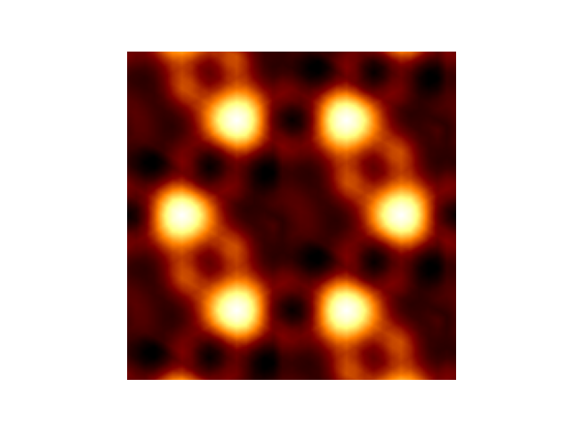
info('Plot scanning-tunnelling image')
plot = elphmod.plot.plot(STM, angle=120)
if comm.rank == 0:
plt.imshow(plot, cmap='afmhot')
plt.axis('off')
plt.savefig('simsts_1.png')
plt.show()
info('Calculate scanning-tunnelling spectrum')
STS = sum(elphmod.dos.hexa2F(e[:, :, n], weight[:, :, n])(w)
for n in range(el.size))
STS *= el.size / (np.sum(STS) * dw)
if comm.rank == 0:
plt.grid()
plt.plot(w, DOS, label='DOS')
plt.plot(w, STS, label='STS')
plt.ylabel('Density of states (1/eV)')
plt.xlabel('Electron energy (eV)')
plt.legend()
plt.savefig('simsts_2.png')
plt.show()