Fluctuation diagnostics
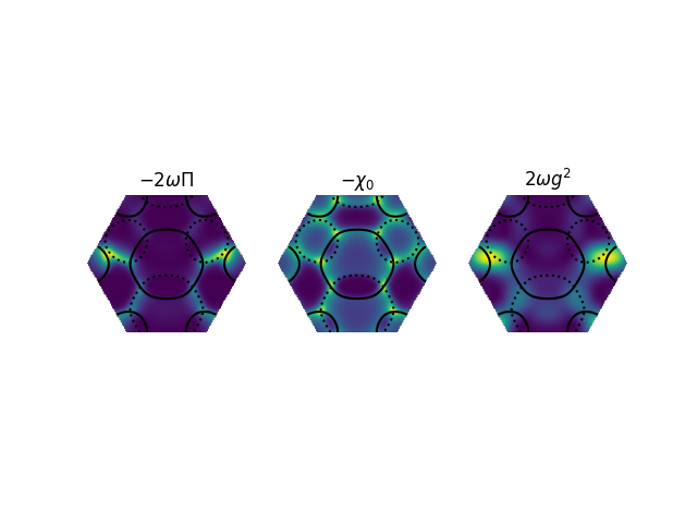
This example will show how to plot the k-resolved phonon self-energy, bare electronic susceptibility, and electron-phonon coupling at the origin of the phonon anomalies and charge-density wave in monolayer 1H-TaS₂ [cf. Fig. 3 (a-c) of Phys. Rev. B 101, 155107 (2020)].
#!/usr/bin/env python3

# Copyright (C) 2017-2026 elphmod Developers
# This program is free software under the terms of the GNU GPLv3 or later.

import elphmod
import matplotlib.pyplot as plt
import numpy as np

comm = elphmod.MPI.comm
info = elphmod.MPI.info

q = np.array([[0.0, 2 * np.pi / 3]])

nk = 48
kT = 0.005

BZ = dict(points=200, outside=np.nan)

info('Load tight-binding model, mass-spring model, and coupling')

el = elphmod.el.Model('TaS2')
mu = elphmod.el.read_Fermi_level('pw.out')
ph = elphmod.ph.Model('ifc', apply_asr_simple=True)
elph = elphmod.elph.Model('work/TaS2.epmatwp', 'wigner.fmt', el, ph)

info('Diagonalize Hamiltonian and dynamical matrix and sample coupling')

e, U = elphmod.dispersion.dispersion_full_nosym(el.H, nk, vectors=True)
e -= mu
e /= elphmod.misc.Ry

w2, u = elphmod.dispersion.dispersion(ph.D, q, vectors=True)

LA = np.argwhere(elphmod.ph.polarization(u, q)[0, :, 0] > 0.5).min()

g2 = abs(elph.sample(q, U=U[..., :1], u=u[..., LA:LA + 1])) ** 2

info('Calculate phonon self-energy and bare electronic susceptibility')

Pi = elphmod.diagrams.phonon_self_energy(q, e[..., :1], g2=g2, kT=kT,
    occupations=elphmod.occupations.fermi_dirac, fluctuations=True)[1]

X0 = elphmod.diagrams.phonon_self_energy(q, e[..., :1], kT=kT,
    occupations=elphmod.occupations.fermi_dirac, fluctuations=True)[1]

info('Map all quantities onto first Brillouin zone')

ek1_BZ = elphmod.plot.toBZ(e[:, :, 0], **BZ)
ek2_BZ = elphmod.plot.toBZ(np.roll(np.roll(e[:, :, 0],
    shift=-int(round(q[0, 0] * nk / (2 * np.pi))), axis=0),
    shift=-int(round(q[0, 1] * nk / (2 * np.pi))), axis=1), **BZ)

Pi_BZ = -elphmod.plot.toBZ(Pi[0, 0, :, :, 0, 0], **BZ)
X0_BZ = -elphmod.plot.toBZ(X0[0, 0, :, :, 0, 0], **BZ)
g2_BZ = +elphmod.plot.toBZ(g2[0, 0, :, :, 0, 0], **BZ)

info('Plot self-energy, susceptibility, and coupling next to each other')

if comm.rank == 0:
    figure, axes = plt.subplots(1, 3)

    for n, (title, data) in enumerate([(r'$-2 \omega \Pi$', Pi_BZ),
            (r'$-\chi_0$', X0_BZ), (r'$2 \omega g^2$', g2_BZ)]):

        axes[n].imshow(data)
        axes[n].contour(ek1_BZ, levels=[0.0], colors='k')
        axes[n].contour(ek2_BZ, levels=[0.0], colors='k', linestyles=':')

        axes[n].set_title(title)
        axes[n].axis('image')
        axes[n].axis('off')

    plt.savefig('fluctuations.png')
    plt.show()