#!/usr/bin/env python3
import ebbw
import numpy as np
import matplotlib.pyplot as plt
N = 101
TcEB = np.empty(N)
TcMM = np.empty(N)
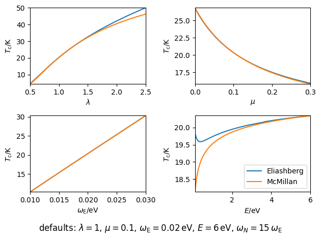
variables = [
('l', np.linspace(0.50, 2.50, N), r'$\lambda$'),
('u', np.linspace(0.00, 0.30, N), r'$\mu$'),
('w', np.linspace(0.01, 0.03, N), r'$\omega_{\mathrm{E}} / \mathrm{eV}$'),
('E', np.linspace(0.10, 6.00, N), r'$E / \mathrm{eV}$'),
]
defaults = dict(T=10.0, l=1.0, u=0.1, w=0.02, E=6.0, W=15.0)
A = 0.94
B = 1.11
C = 0.74
A *= ebbw.Tc(**defaults, A=A, B=B, C=C)
A /= ebbw.critical(**defaults)
figure = plt.figure()
for position, (key, x, label) in enumerate(variables, 221):
parameters = defaults.copy()
for i, parameters[key] in enumerate(x):
print('%s = %g' % (key, parameters[key]))
TcEB[i] = parameters['T'] = ebbw.critical(**parameters)
TcMM[i] = ebbw.Tc(**parameters, A=A, B=B, C=C)
plt.subplot(position)
plt.autoscale(tight=True)
plt.plot(x, TcEB, label='Eliashberg')
plt.plot(x, TcMM, label='McMillan')
plt.xlabel(label)
plt.ylabel(r'$T_{\mathrm{c}} / \mathrm{K}$')
plt.legend()
plt.suptitle(r'defaults: '
r'$\lambda = %(l)g$, '
r'$\mu = %(u)g$, '
r'$\omega_{\mathrm{E}} = %(w)g\,\mathrm{eV}$, '
r'$E = %(E)g\,\mathrm{eV}$, '
r'$\omega_N = %(W)g\,\omega_{\mathrm{E}}$'
% defaults, y=0)
plt.tight_layout()
figure.savefig('mcmillan.png', bbox_inches='tight')